Tutorial
To demonstrate MAVEN we will be using a dataset from Sun et al., GEO accession GSE129254 which is found in Example_Data/lapatinib. The filetree structure of the folder is shown below:
Example_Data/
├─ lapatinib/
│  ├─ CARNIVAL_results/
│  │  ├─ carnival_result.RDS
│  │  ├─ network.sif
│  ├─ target_prediction_results/
│  │  ├─ PIDGIN_out_predictions.txt
│  │  ├─ PIDGIN_similarity_details.txt
│  ├─ get_data.R
│  ├─ GSE129254_lapatinib_BT474.txt
│  ├─ lapatinib.txt
The gene expression data is contained in GSE12954_lapatinib_BT474.txt and was generated using the get_data.R script. The data represents the response of BT474 cells following treatment with Lapatinib in terms of the t-statistic compared to control (DMSO-treated BT474 cells). The compound SMILES are contained in lapatinib.txt.
To start, set the MAVEN directory as the working directory in RStudio, call renv::restore(), and then shiny::runApp(). In a few seconds, the app should have loaded. Please ensure you carefully read the installation instructions before completing the tutorial.
Step 1. Data
To begin the analysis, click on the 1. Data button in the top toolbar. In this step, the prior knowledge network and gene expression data are uploaded.
The gene expression data will be used in 3. Analysis with DoRothEA to infer transcription factor activities, and with PROGENy to infer pathway activities. The transcription factors are used as input to CARNIVAL, along with the protein weights as defined by the pathway activities, and the prior knowledge network.
To load the example data, click on the “Load example network” and “Load example data” buttons. This will load the files Example_Data/omnipath_full_carnival.sif and Example_Data/lapatinib/GSE129254_lapatinib_BT474.txt.
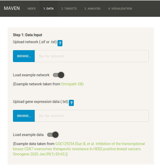
Alternatively, you can upload the two files manually. NB a check is performed to make sure all gene symbols are valid. Any invalid symbols will be written to a log file in the logs/ folder of the main MAVEN directory.
Now move on to 2. Targets.
Step 2. Targets
Targets are optional in MAVEN, and it is possible to perform the CARNIVAL analysis without defining targets. For this tutorial, we will be predicting the targets of Lapatinib using its chemical structure. It is also possible to skip the prediction step and define targets if they are known beforehand.
In MAVEN, target prediction is carried out with PIDGIN, which is essentially a collection of pre-trained models (one for each protein target contained in ChEMBL). Only human targets are predicted in MAVEN.
The Targets tab contains 4 sub-tabs - (A) Upload SMILES (B) Run options (C) Results (D) User-defined targets.
(A) Upload SMILES
In the (A) Upload SMILES tab, load the Lapatinib SMILES by clicking on the toggle. Check that the structure is correct by viewing the rendered compound image. You can also manually upload the SMILES file Example_Data/lapatinib/lapatinib.txt.
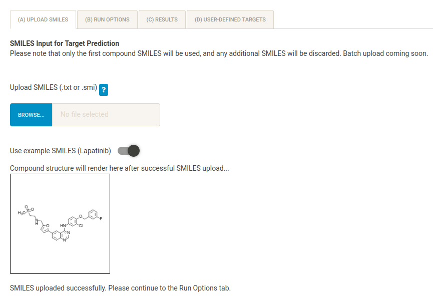
NB If you don’t know your compound’s SMILES, it is possible to generate a SMILES file by sketching the compond structure in the applet and clicking “Get SMILES”.
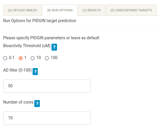
(B) Run options
In the (B) Run options tab you can define several different options. For target prediction, compound bioactivities are binarised at different thresholds (0.1, 1, 10 and 100 uM). The default threshold used to generate predictions is 10 uM. Because the Lapatinib gene expression data were measured at 1 uM, change this option to 1.
Predictions derived from machine learning models cannot be trusted if the query compound is very dissimilar to the componds used to train the models - known as being outside of the “Applicability Domain” or AD of the models. Hence, AD percentiles (0-100) are computed using the Reliability Density Neighbourhood methodology and used to filter the predictions. For each model (target), if the computed AD percentile falls below the defined threshold (here 50), the prediction is not output. To obtain more prediction (but potentially less realible) decrease the AD filter and vice versa. To turn off the AD filter altogether, you can input 0 for this option. For this tutorial, keep the AD threshold to its default value.
It is possible to parallelise the target prediction over a number of cores. You can change this number to one that is appropriate for your machine.
Finally, browse to select the PIDGIN installation directory (the folder containing the predict.py file). You can type in a filepath using the pencil symbol on the file browser.

To run the target prediction, press the RUN PIDGIN button. This may take a while depending on how many cores are being used, and you can check the progress by monitoring the console in R Studio.
Once the predictions have finished running, the (C) Results page will be populated. In the output/ folder of the main MAVEN directory, a directory will be created containing the output files from the target prediction, as well as a file containing the corresponding command line operation, to keep record of the parameters used to generate the predictions.
(C) Results
The (C) Results page will display the target prediction results when they are obtained.
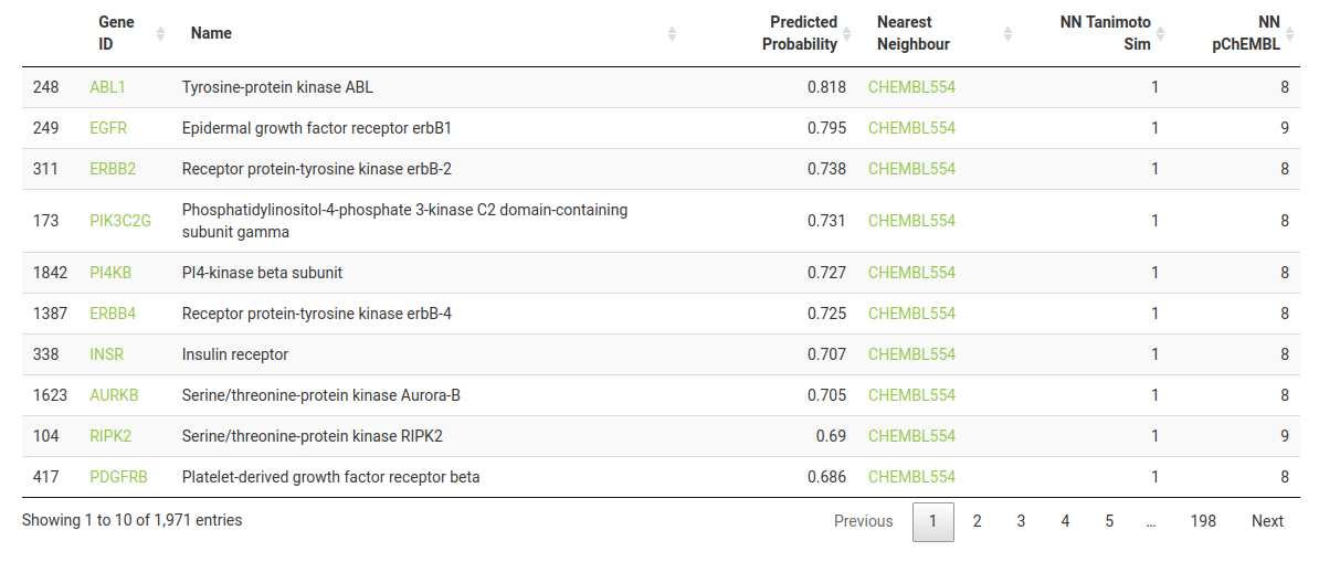
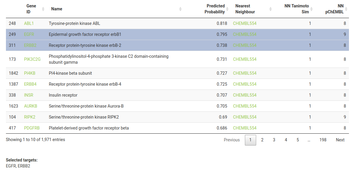
By default, the results table is sorted by probability of activity (descending). The columns represent the following:-
Gene ID -> Target HGNC symbol - you can click to take you to the corresponding UniProt entry for more information on the protein’s function.
Name -> Target preferred name.
Predicted Probability -> Probability (between 0 and 1) of activity at the defined bioactivity threshold.
Nearest Neighbour -> ChEMBL ID of the most structurally similar compound in the target’s training dataset. You can click to take you to the corresponding page on ChEMBL.
NN Tanimoto Sim -> Tanimoto Similarity (between 0 and 1) of the Nearest Neighbour compound compared to the query compound.
NN pChEMBL -> pChEMBL (bioactivity) value for the Nearest Neighbour for the particular target. pChEMBL is defined as -log10(XC50).
You will notice that many of the targets have a value of 1 for NN Tanimoto Sim. This means that Lapatinib itself was part of the training set - click on the ChEMBL link (ChEMBL554) to see for yourself.
For this tutorial, we are investigating the cellular response of HER2-positive BRT474 cell line to the modulation of EGFR and ERBB2 by Lapatinib. Select the corresponding rows, such that they are displayed under Selected targets below the table.
It is also possible to upload the output from a previous run. In Example_Data/ there is a folder entitled target_prediction_results/. This contains the predictions (PIDGIN_out_predictions.txt) and the similarity analysis (PIDGIN_similarity_details.txt) from the Lapatinib results using the above parameters. When uploading results, please select BOTH files to populate the page.
(D) User-defined targets
For the purpose of the tutorial, leave this blank. If you know your query compound’s targets then it is possible to skip the target prediction altogether and click on this tab to directly input the target HGNC symbols.
Step 3. Analysis
Now we have all of the information we need to begin the analysis. The 3. Analysis tab contains 3 sub-tabs - (A) DoRothEA (B) PROGENy (C) CARNIVAL. Options for each of the steps can be modified in the side-panel.
(A) DoRothEA
For DoRothEA transcription factor (TF) enrichment there are two options. The first, Confidence levels, defines which TF-gene regulons will be used to perform the enrichment (where A is most confident and E is least confident). For more information on confidence levels, refer to the DoRothEA documentation. Keep the defaults (A, B and C).
The second option defines the number of TFs to be used as input for CARNIVAL. Keep the default (50).

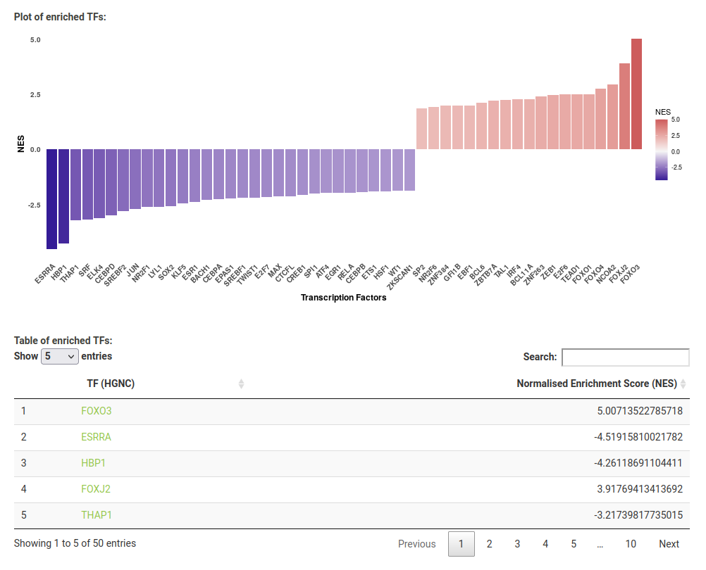
Click “RUN DOROTHEA” and the page will be shortly populated with a plot and results table.
The plot and table display the HGNC symbol for each enriched TF with its normalised enrichment score (NES). A positive NES indicates an upregulation of the TF, and negative indicates a downregulation. You can click on a symbol in the results table to take you to the corresponding UniProt page. Note that the top upregulated TF, FOXO3, is known to be activated by Lapatinib ref and the top downregulated TF, ESRRA, is known to be degraded by Lapatinib ref.
You can also save the results (plot image, results table and parameter log) to your machine with the Download button.
(B) PROGENy
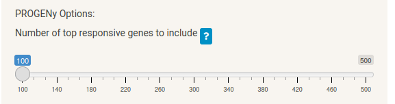
For PROGENy there is only one option; the number of top responsive genes to include in the pathway activity calculation. The default (100) should be suitable for most cases.
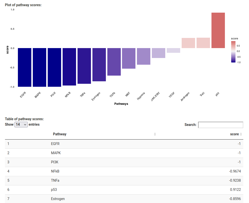
Press “RUN PROGENY” and the page will be shortly populated with a plot and results table.
The plot and table display the pathway activity score for each of the 14 pathways contained in the PROGENy methodology, where again a negative score indicates downregulation and a positive score upregulation. Though you may not deem these specific 14 pathways as relevant to your compound, the purpose of this step is to improve the CARNIVAL network optimisation results by pre-weighting a set of proteins in the prior knowledge network.
Like with DoRothEA, you can save the results to your machine with the Download button.
(C) CARNIVAL
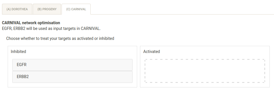
For CARNIVAL there are four settings in the side-panel. The targets selected in 2. Targets are displayed and can be unchecked or checked. Leave both EGFR and ERBB2 checked.
You can also set a time limit for the CARNIVAL run, though decreasing this too much may mean that an optimal solution is not found. Leave this value as the default 3600 seconds.
When using the IBM ILOG CPLEX solver it is possible to parallelise the calculations over a number of cores. Change this value to one appropriate for your machine. Note that for this tutorial, 20 cores were used.
CARNIVAL can be run with the IBM ILOG CPLEX solver (free for academic use), the Cbc solver (free) and lpSolve (free). All solvers except for lpSolve must be pre-installed. We recommend that you use IBM or Cbc solvers for real-life cases, as lpSolve only works for smaller, toy examples. For this tutorial, the IBM ILOG CPLEX solver was used.

In the main panel, you can select the direction (activated/inhibited) of your chosen targets. Leave both as inhibited (default), as Lapatinib is known to inhibit EGFR and ERBB2.
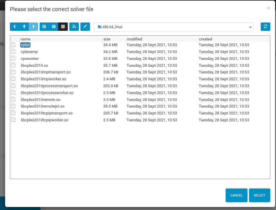
Finally, you must select the solver file - for the IBM ILOG CPLEX solver this is usually ibm/ILOG/CPLEX_StudioXXXX/cplex/bin/OS_specific_folder (e.g. x86-64_linux)/cplex.
Click “RUN CARNIVAL”, this may take a while. When CARNIVAL has finished running, the results (an .RDS file which can be loaded into the app on the next page, and a .sif file containing the network which can be opened in your favourite network visualisation software) will be saved in a folder along with a log file with all of the parameters used to generate the output (including DoRothEA and PROGENy settings). The resulting network will also be displayed on the 4. Visualisation page.
Step 4. Visualisation
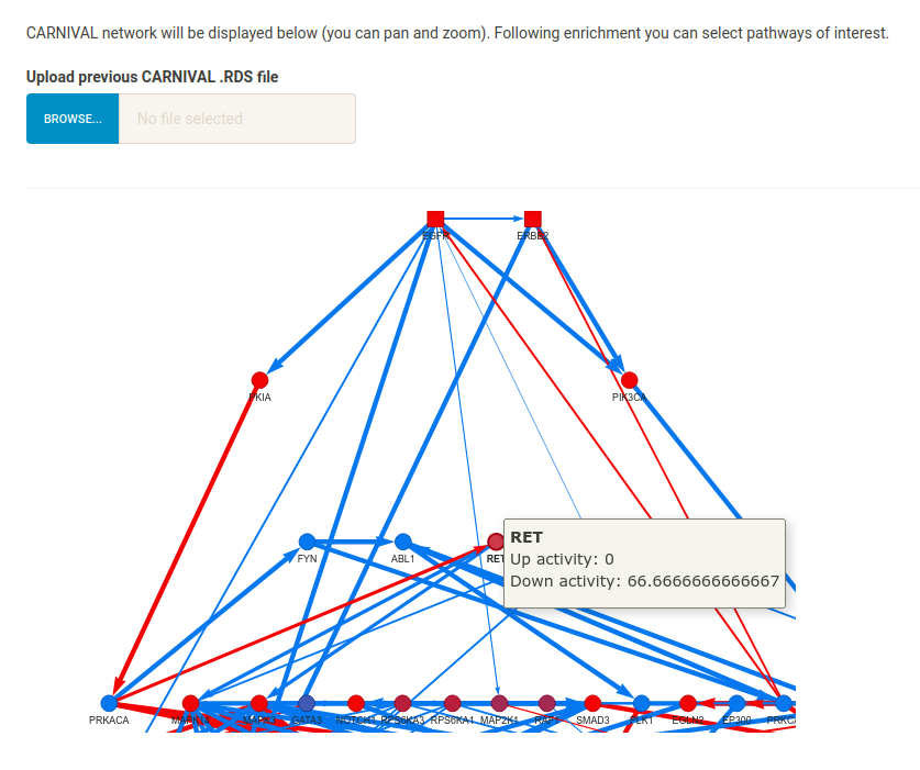
When CARNIVAL has finished running, the resulting network will be displayed in the main panel. You can also upload a previous result (the .RDS file saved in the relevant output/ folder after a CARNIVAL run). To upload the resulting Lapatinib network based on the tutorial settings, navigate to Example_Data/lapatinib/CARNIVAL_results/carnival_results.RDS. Note that your results may look slightly different depending on the solver, time-limit and number of cores used. The rest of this section assumes that you have loaded the results from the tutorial files.
Notice that the network has connected the input targets (square nodes) to the input TFs (triangular nodes) via signalling proteins from the prior knowledge network. Nodes are coloured red (down-regulated) or blue (up-regulated) depending on their pre-set (targets, TFs) or inferred (intermediate signalling proteins) regulation. Because multiple solutions are found and combined to produce the final result, some nodes may not be inferred as always up- or down-regulated in every solution. For example, hover over RET - this node has a down-regulation of 66.6* because it was inferred as down-regulated in 2/3 of the total solution pool.
Because the network represents inferred signalling proteins modulated by Lapatinib, we can perform pathway enrichment to understand which specific pathways may be modulated by the compound (which could inform on which experimental assays to perform to validate the compound’s MoA).
The side-panel allows you to choose from pre-defined MSigDB gene set collections, or use a custom .gmt file. You can choose to keep or discard the input TFs from the enrichment analysis - this is because including TFs can sometimes lead to an over-abundance of transcription-related pathways. Click “RUN ENRICHMENT ANALYSIS” with the default settings (Hallmark collection, include TFs) and a results table will shortly be displayed in the main page.

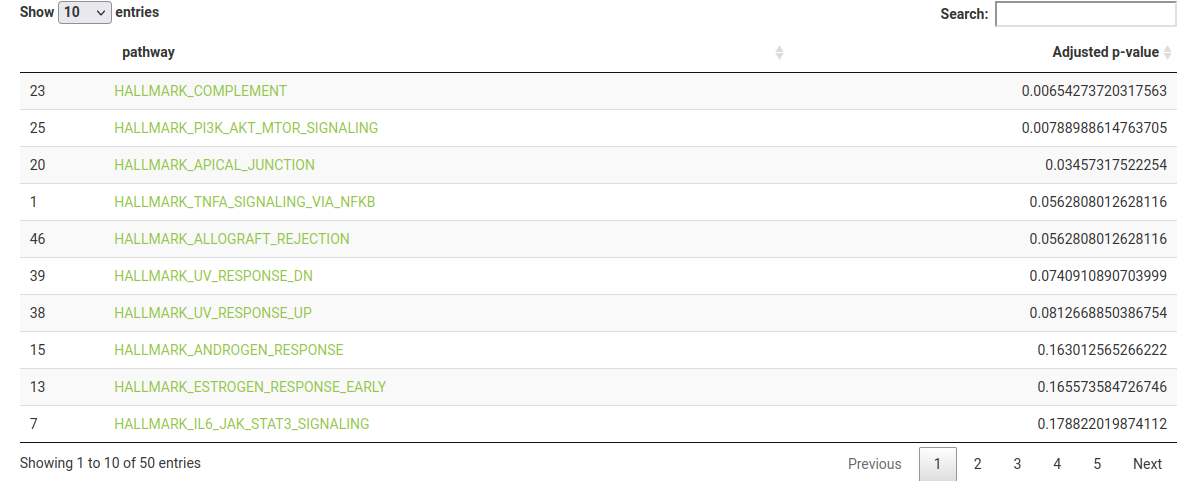
The results table displays the pathway name (with a link to the corresponding gene set on MSigDB, if one of the built-in gene set collections are used) and the BH-adjusted p-value. You can download the full pathway enrichment results to your machine with the Download button.
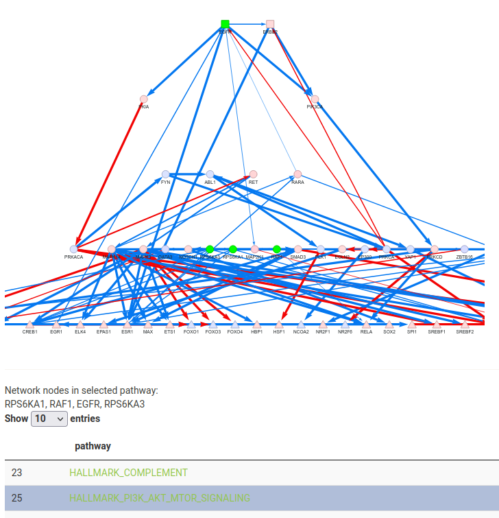
Note that HALLMARK_PI3K_AKT_MTOR_SIGNALLING is significantly enriched (adjusted p-value = 0.008), and was found to be modulated by Lapatinib in the dataset’s publication.
You can click on a row in the results table to output the specific network nodes in the gene set, and to light them up on the network.
Next Steps
This is the end of the tutorial - if there were any issues, get in touch (lh605[at]cam[dot]ac[dot]uk). If you decide to use MAVEN to analyse your own data, please cite our preprint.